Use StatsD to Measure Your Python App Metrics

If you’re a fan of DevOps, then you should also be enthusiastic about collecting telemetry from your production applications. StatsD is one solution that you could use to collect metrics in Python.

Application telemetry gives you the visibility to what’s happening in your production system, and it enables you to solve problems when something inevitably goes wong. Log entries and exceptions are usually enough to debug many issues, but with application metrics you might be able to spot emerging problems faster, before they actually impact the customer.

Uncovering issues is not the only use case for collecting metrics. They can also help you to understand how people are using your service. You could track usage across different APIs to find what features people use the most or how many people log in to your product each day. Increased response times might mean that you need to allocate more compute resources to your service.

The data could help you prioritize work on the most important features, and it can enable you to experiment with A/B testing.

What is StatsD?

StatsD is a network daemon that listens to events from different sources using a simple UDP or TCP based protocol. It can forward these events to visualization platforms, such as Grafana.

It was originally written at Etsy where they were really enthusiastic about collecting statistics and drawing graphs. They wanted a solution that would let developers collect this data with minimal development effort. Here’s the blog post about the reasonings and design choices that they made.

Stats are collected in buckets. Each bucket contains one statistic, and they are not preconfigured. Instead, they are genereated on the fly as events are pushed to the server.

Metrics are sent with values which are typically integers. The flush interval defines how often these values are aggregated and sent forward to the stats backend service. By default, updates are pushed out every ten seconds.

If your application is instrumented with metrics collection it can send events when some functions are called. A practical example could be an API endpoint that increments a hit counter each time it is called and sends the amount of time it took to process the request.

It is recommended that you configure the stats collection using the UDP protocol since it is a fire and forget type of communication, and will therefore have smaller effect on the application performance. A TCP connection requires a three-way handshake initialization, which means that it could potentially affect your app performance if you’re collecting lots of stats.

Still, if you’re sending lots of stats to an external system the physical network interface might actually become the limiting factor to your app’s performance. So keep that in mind if you encounter performance issues.

Set up StatsD and Graphite

Since StatsD doesn’t come with its own visualization system to graph the metrics you’d typically want to pair it with something like Graphite. In this equation StatsD will gather and aggregate single data points while Graphite stores and renders the numeric time-series data.

The easiest way to run StatsD and Graphite together locally is to use the official Docker container from Graphite. The Docker Hub page describes the usage quite well, note that you should mount the configuration volumes to a known location in your host machine if you want to change any configurations.

Make sure that you have Docker installed on your machine. Now you can use the following command to download and start the container locally:

docker run -d\
 --name graphite\
 --restart=always\
 -p 80:80\
 -p 2003-2004:2003-2004\
 -p 2023-2024:2023-2024\
 -p 8125:8125/udp\
 -p 8126:8126\
 graphiteapp/graphite-statsd

The command starts the container in the background, names it graphite and binds all the needed ports. After the command has run successfully you should be able to see the running container with the docker ps command.

If you’d wish to configure multiple containers you could also use the statsd/statsd image. Then you would also need to configure the networking between your visualization container, and so on. That is out of the scope of this article.

If everything went smoohtly, you should now be able to access the Graphite web UI from http://localhost.

Create a Python application

Let’s create a simple API that we can call from a browser. We’re going to use the FastAPI framework that makes API development really easy. It requires Python 3.6 or newer. I’m not going to go too deep into FastAPI so I will keep this example quite simple. I recommend that you check out their documentation in case you’re interested to learn more about it.

Let’s start by creating a new directory, setting up the virtual environment, and installing the requirements:

mkdir statstest
cd statstest
python3 -m venv venv
. venv/bin/activate
python3 -m pip install fastapi uvicorn

Here FastAPI is our API framework and Uvicorn acts as the ASGI server that actually runs the code and handles the incoming connections.

Next, implement the API and save it as main.py:

from fastapi import FastAPI

app = FastAPI()

@app.get("/")
def root(msg: str = None):
  	if msg:
        return {"message": msg}
    return {"message": "No message provided!"}  

If you’re familiar with Flask then this should also feel familiar to you. The code defines a GET endpoint using a decorator that configures the URL path. The decorated function accepts a single argument called msg, which is automatically interpreted as a query argument. The API responds with a JSON message that contains the same text that it was given.

You can start the development server with this command:

uvicorn main:app --reload

The reload flag makes uvicorn watch the directory for code changes.

Now you should be able to access the API by accessing http://localhost:8000 with your browser. The response should say that you didn’t provide a message. Define a message as the query argument and verify that it works. You can use plus signs as space, for example http://localhost:8000?msg=Hello+world. Your browser should now show:

{"message":"Hello world"}

You should also see the request appear in the Uvicorn logs on the command line.

Instrument your application

Next you need to start sending events to the StatsD daemon. Install the statsd package with this command:

python3 -m pip install statsd

There are different ways that you can configure the StatsD client connection but since we have the daemon running locally under the default port we don’t need to configure anything manually. All configuration options are explained in the Python StatsD documentation but we’re going to use the environment variable setup. This would work well for serverless setups where configurations for containerized applications are often provided through environment variables.

Counters

Let’s start collecting some stats. Counters are metrics that can be used to measure the frequency of something. The following code imports the statsd client and then uses the incr method to increment a counter.

from fastapi import FastAPI
from stasd.defaults.env import statsd

app = FastAPI()

@app.get("/")
def root(msg: str = None):
    statsd.incr("statstest.root.called")
  	if msg:
        return {"message": msg}
    return {"message": "No message provided!"}  

You need to provide the name of the counter that you want to increment, this will automatically create the matching entry on the stats server. Dots can be used to create directory hierarchies. You can also use the decr method to decrement a counter.

The optional second argument can be used to increment the counter by more than one. So if your code is already combining counts you can report them in a batch. For example:

statsd.incr("statstest.root.called", 10)  # increment by ten

Refresh the browser window with the API call a few times to generate artificial load and go back to the Graphite UI. If you refresh the tree view you should see that the new statistic has appeared in the stats folder as seen in the image below.

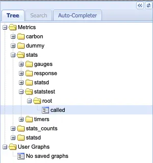
You can add this data to a graph view to see how the values change over time. Your graph may look a little bit different from mine since I have made some configurations to the visualization.

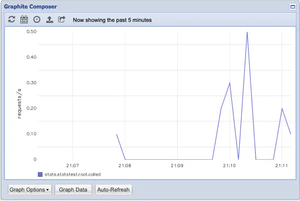
Counters might feel a bit counter-intuitive at first when you look at them in Graphite but their logic is actually quite reasonable. Since StatsD is aggregating the counter values over ten seconds (the default), the values are sent as events per second over the aggregation period. If you called the API only once within a ten second time period the graph would show 0.1 instead of 1.

So remember that it is not actually counting event occurrences but the frequency of events within the sampling period.

Timers

Timers are your best friend when you need to monitor execution times of functions in your code. The timer decorator can be used to wrap a function call, and it will automatically create statistical values on the monitoring backend.

The following code adds a random sleep to the function which emulates heavy processing that could take a varying amount of time. The API function is also wrapped with the @statsd.timer decorator that handles all the heavy lifting for us. Note that the order of the decorators matters here!

from fastapi import FastAPI
from stasd.defaults.env import statsd

import time
import random

app = FastAPI()

@app.get("/")
@statsd.timer("statstest.root.timer")
def root(msg: str = None):
    time.sleep(random.uniform(0, 0.5))
  	if msg:
        return {"message": msg}
    return {"message": "No message provided!"}  

If you want to generate the test data without manually refreshing the browser window, you can call curl in a loop. This command waits for one second between API calls, and it should work directly on Linux and macOS:

while sleep 1; do curl "http://localhost:8000/?msg=Hello+world"; done

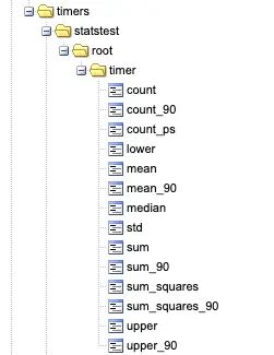
Now that you’ve called the API with the new timer code you should see the corresponding entry in the Graphite tree view under the timers section. As you can see, there are quite many values that have been automatically calculated for you.

Often, it is interesting to plot the averages of response times. In some edge cases client requests might take a lot longer to process than expected while most of the users are happily using the service without noticing anything weird. The mean_90 and upper_90 strike a balance between monitoring how the majority of users experience the service while filtering out outliers as they only take the lowest 90 percentile into account.

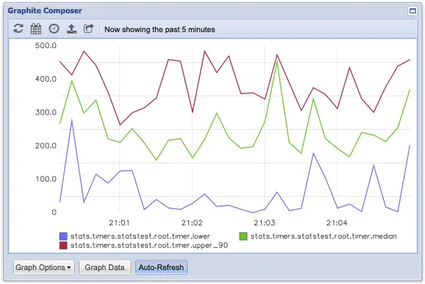
The graph above contains the median, upper 90, and lowest values for the root timer during the last five minutes. The reported values are in milliseconds.

You can also observe the standard deviation, sum, sum of squares, and count of events. In this case count is actually the real observed count of events within the sampling period, not the rate of requests as we saw with the counter.

Gauges

Gauges show constant values. When you set a gauge, it will draw a flat line on the graph until you change the value to something else. Therefore it is a good solution for data that doesn’t need to be reset or averaged over time, such as system load or RAM usage.

The usage is similar to the previous examples:

statsd.gauge("my-server.resources.memory", 4128)

The gauge supports an additional delta argument. If you set it to true the gauge value will change relative to the current value instead of setting an absolute value. However, you should remember that it is possible that some network packages may be lost which could make the value inaccurate over time. So it is best to use absolute values whenever possible.

Another pitfall with gauges is that if your service stops sending messages due to an error the gauge value will not reflect this since the monitoring server still remembers the last value it has seen. Do not use a gauge as the only signal to verify that a service is up and running!

Sets

In mathematics a set is a collection of distinct elements. The same is true with StatsD. You can use a set to count the number of unique values, such as unique users calling your API during the sample period.

Let’s create another dummy endpoint that can be used to query user data, and which uses a set to log the number of distinct users based on the user ID. (You can add this to your existing program.)

@app.get("/user")
def get_user(id: int):
    statsd.set("statstest.user", id)
    return {"id:" id}

Now you can call http://localhost:8000/user?id=123 with different id values. Then, the data can be graphed from the stats.sets.statstest.user.count metric on Graphite.

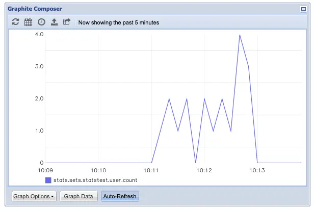
If you call the enpoint many times with the same value you will see that the graph stays at one during the sample period. When you change the value of the ID argument you’ll notice that the graph shows the amount of unique IDs within each ten second time period.

Final thoughts

Hopefully this post gave you a good start on using StatsD with Python. As you can see it is not very difficult to start collecting application metrics. On the code level it is usually only one line of code that needs to be added to the correct place.

The real difficulties start when you start configuring the stats server and graphs. When you dig deeper you might encounter strange issues with how the systems interact with each other or how they aggregate the data over different time spans. Then it is best that you spend some time reading the official documentation to understand what is happening.